GreenFlux

A greenhouse simulator whose physics you can trace, calibrated against measured data.

GreenFlux models greenhouse climate — air temperature, humidity, CO₂ — together with tomato crop growth, the equipment that drives them, and the economics of running the whole thing. It exists to answer questions that need a plant you can trust: control strategies, dataset generation for ML, anomaly and fault studies, sensor observability.

Where the numbers stand

Validated against the GreenLight Bleiswijk measured-replay dataset, out of sample — the calibration is fitted on one window and scored on the others.

Over 14 strided one-day periods across the 112-day season, on the measured_replay profile:

installation	air temperature	relative humidity	vapour pressure	CO₂
LED	2.17 °C	8.17 %	252 Pa	101 ppm
HPS	2.34 °C	9.93 %	274 Pa	65 ppm

Over 13 seven-day windows, on measured_replay_physical — the profile projects now select by default, with physical parameters rather than curve-fitting fudges:

installation	air temperature	relative humidity	vapour pressure	CO₂
LED	2.00 °C	7.34 %	256 Pa	unidentifiable
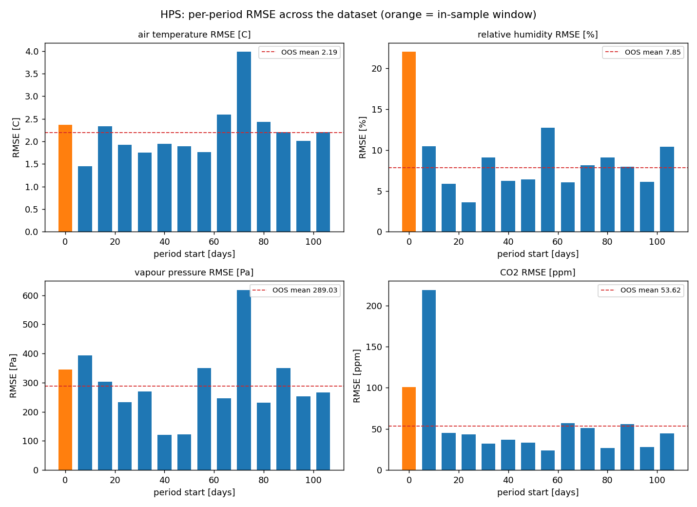
HPS	2.19 °C	7.85 %	289 Pa	54 ppm

Both profiles sit under the project's 2.5 °C acceptance target, and they are different audits rather than competing estimates — different windows, different profile. Which to quote depends on which profile you run; see physical models.

CO₂ is a diagnostic, not a prediction. The dataset's injection signal is a binary status flag rather than a flux, off 97 % of the time while CO₂ is dosed to ~780 ppm. HPS lands where it does because its dosing gain is identifiable; LED's is not.

What the validation looks like

Each bar is one replay window. Orange is the single window the calibration was fitted on; the dashed line is the mean over the windows that were not. Reported this way because a single in-sample window is not evidence — earlier one-day figures of ~2 °C degraded to 15–22 °C when replayed elsewhere in the season.

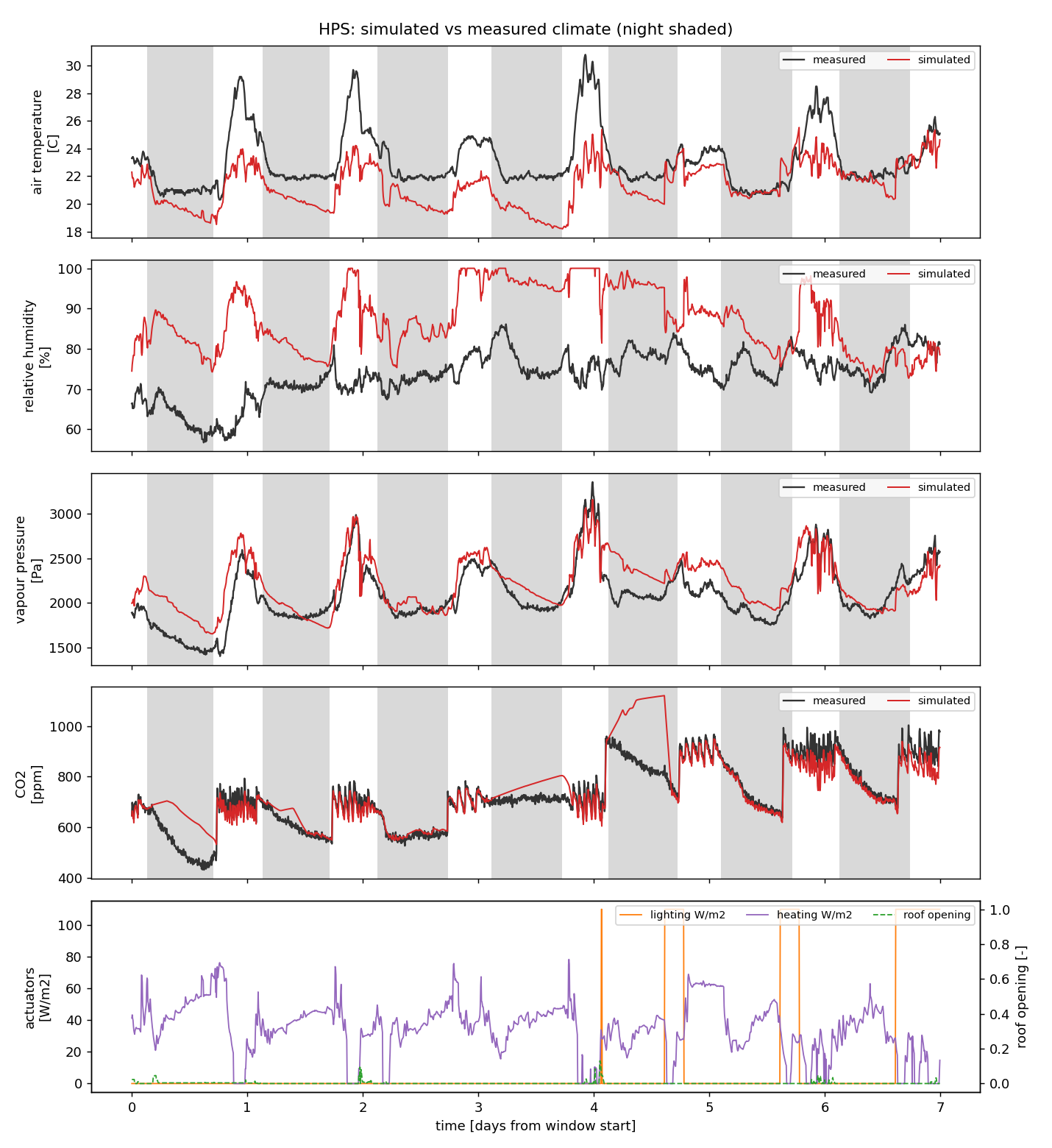
And what a replay looks like over seven days, including where it is wrong — CO₂ and vapour pressure track closely, air temperature runs about 2 °C cold and clips the daytime peaks, and relative humidity is biased high enough to saturate. Both biases are open and traced to the lumped heat balance, not to calibration.

Regenerate the whole set with:

uv run --extra plots python examples/plot_validation.py --installation HPS

What you probably want

• Define a greenhouse

  Geometry, envelope, equipment, crop and weather in one declarative project.json.

  Start with projects

• Run a simulation

  Closed-loop climate control with heating, ventilation and CO₂ dosing.

  Forward mode

• Ask a research question

  Declarative studies over a project — planning under uncertainty, anomaly detection, control.

  Studies

• Understand the model

  Which physical models exist, what they assume, and what they deliberately do not model.

  Physical models

How it fits together

Layers depend downward only. The boundary is enforced by an architecture test, so a physics module cannot start importing project or analysis code.

flowchart TB
    EQ["<b>equations</b><br/>scalar physics primitives<br/><small>psychrometrics · fluid flow · heat transfer</small>"]
    FL["<b>flows</b><br/>coupled transfer<br/><small>ventilation · transpiration · condensation</small>"]
    EQP["<b>equipment</b> · <b>components</b><br/>actuators and passive elements<br/><small>heating · vents · CO₂ · screens · lamps</small>"]
    CR["<b>crop</b><br/>staged tomato growth<br/><small>photosynthesis · partitioning · fruit</small>"]
    SY["<b>systems</b><br/>the assembly<br/><small>GreenhouseUnit · state derivatives</small>"]
    SI["<b>simulators</b><br/>fixed-step · adaptive IVP"]
    PR["<b>projects</b><br/>declarative definition · calibration profiles"]
    AN["<b>analysis</b> · <b>studies</b><br/>validation · calibration · research questions"]

    EQ --> FL
    EQ --> EQP
    FL --> SY
    EQP --> SY
    CR --> SY
    SY --> SI
    SI --> PR
    PR --> AN

    style SY fill:#00695c,stroke:#004d40,color:#fff
    style EQ fill:#26a69a,stroke:#00796b,color:#fff

systems is the load-bearing layer: every physical term that contributes to a state tendency is a named field on a flux record, which is what makes balance decomposition and per-term calibration possible without changing the model's shape.

What a run actually does

sequenceDiagram
    autonumber
    participant P as project.json
    participant B as builder
    participant W as weather + controls
    participant U as GreenhouseUnit
    participant S as solver
    participant R as results

    P->>B: geometry, equipment, crop, calibration profile
    B->>U: build a unit with the profile applied
    loop every step
        W->>U: outside climate, setpoints, actuator commands
        U->>U: solar · heating · ventilation · transpiration · condensation
        U->>S: state derivatives + a full flux record
        S->>U: integrated next state
    end
    S->>R: trajectories, consumption ledger, clipping diagnostics

Two solver paths share the same physics: a deterministic fixed-step Euler driver, and SciPy's adaptive solve_ivp. Which to use, and why it matters, is in choosing a solver.

The two timescales

Greenhouse decisions split across timescales that differ by three orders of magnitude, and the software follows that split rather than fighting it.

flowchart LR
    subgraph slow["Slow layer — days to a season"]
        PL["planning<br/><small>setpoint trajectories, contracts</small>"]
    end
    subgraph fast["Fast layer — minutes to hours"]
        CT["climate control<br/><small>heating, vents, CO₂</small>"]
    end
    subgraph plant["Plant"]
        GH["GreenhouseUnit<br/><small>climate + crop states</small>"]
    end

    PL -->|setpoints| CT
    CT -->|actuation| GH
    GH -->|realised climate and yield| PL
    GH -->|measured state| CT

    style PL fill:#00695c,stroke:#004d40,color:#fff
    style CT fill:#26a69a,stroke:#00796b,color:#fff

A note on how results are reported here

This project has repeatedly found that control conclusions drawn from a simulator are fragile to how the simulator is specified. One metric was measured six times while modelling defects were fixed, moved by more than twice its own effect size, and ended at statistically zero.

What survived that was not a better optimiser but a better question: results measured as constraint satisfaction held, where results measured as expected margin did not. The study pages say which kind each result is, and quote the caveats next to the headline rather than in a footnote.